
Recovery of Implied Uncertainty for Ambiguity Averse Agent
Published:
Introduction:
Within Psychological and Economics research there are two main kinds of uncertainty, risk, in which the probabilities associated with an outcome are known, and ambiguity, in which the probabilities associated with an outcome are unknown (Bland, & Schaefer, 2012). Early theories about decisions under ambiguity suggested that when risks are unknown people behave ‘as though’ they assign numerical probabilities, or “degrees of belief,” onto the outcomes and treat ambiguous outcomes as having the assigned risks (Ellsburg, 1961). However, the classical Ellsberg paradox [ 1 ] showed this could not be true. When asked to choose, participants strongly preferred to bet on the outcome of flipping a coin heads (i.e. a probability of 50%) to picking a blue ball or a red ball from an urn with an unknown concentration of red and blue balls. If participants behaved ‘as though’ they assign numerical probabilities to these outcomes it would suggest that they thought the probability of pulling a red ball and a blue ball were both less than 50%, which cannot be true. Consequently, most psychological studies have either only measured ambiguity aversion as a behavioral bias (Gilboa, 2025).Yet understanding how people form and act upon beliefs is an important line of psychological inquiry, with broader psychological phenomena, including emotional regulation, psychiatric symptoms, and developmental change in uncertainty processing. However, formalizations of ambiguity aversion and computational modeling could allow for some insight into these beliefs.
Formalization of behavior through computational modeling has gained recent popularity (Palmintiri et al., 2017 TICS) and been a boon within the fields of psychology and neuroscience for two reasons which create a virtuous cycle. Models of ambiguity aversion, largely using the max–min expected utility (MMEU) framework (Gilboa and Schmiedler,1989; Levy 2012), have been used to link ambiguity preferences to psychiatric conditions such as PTSD, substance use, anxiety, and autism, as well as to developmental differences (e.g., adolescent risk taking), personality traits (Buckholtz, 2017), and biological measures including BOLD responses, sympathetic arousal, and hormonal or electrophysiological indices. However, this approach means that we cannot recover the agents beliefs about the uncertainty from their decisions. Developing a Bayesian implementation of the KMM recursive expected utility model that allows recovery of both subjective probability beliefs and ambiguity tolerance directly from choice behavior.
Methods:
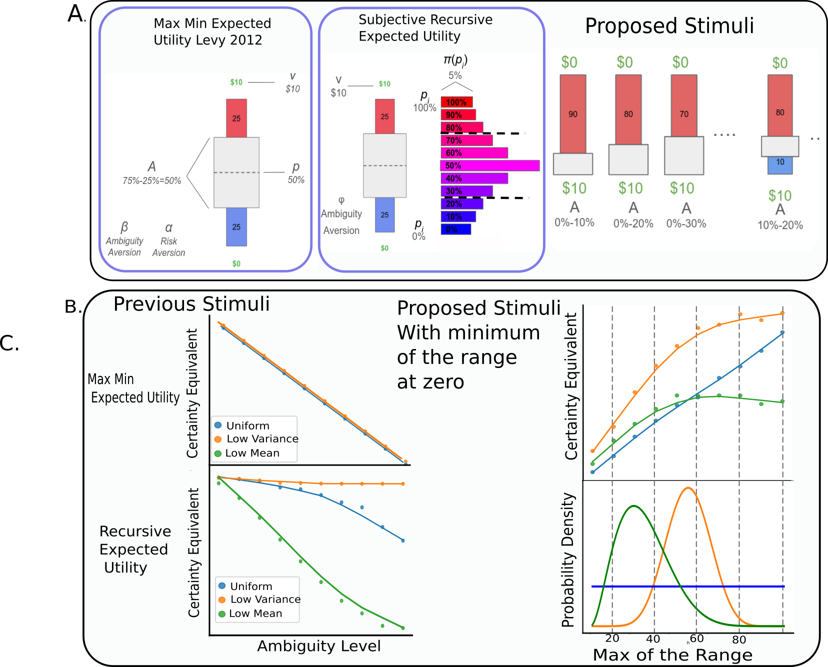 _Figure 1: Typical stimuli for ambiguous lotteries and the interpretation of different model parameters under MMEU and REU. B.) A set of proposed stimuli. Notice that both the widths and midpoints of the “mask” varies throughout the experiment. C.) Ambiguity averse decision behavior using masks centered at 50% under the MMEU and REU rules. Under MMEU all second order distributions are valued the same and the certainty equivalent decreases linearly with the Ambiguity level A, (i.e. the range of the centered “mask”). Under REU the change in the CE is non-linear from interactions of the preference phi and the local shape of the underlying distribution. D.) Under the REU regime in an experiment where the bottom of the range is 0% the certainty equivalent _
$C.E.= [ \Sigma_i (v \times \pi_i)^ \phi_s \times Pr( \pi | Beta( \alpha_b , \beta_b ) ) ] ^ (\phi/s) $ 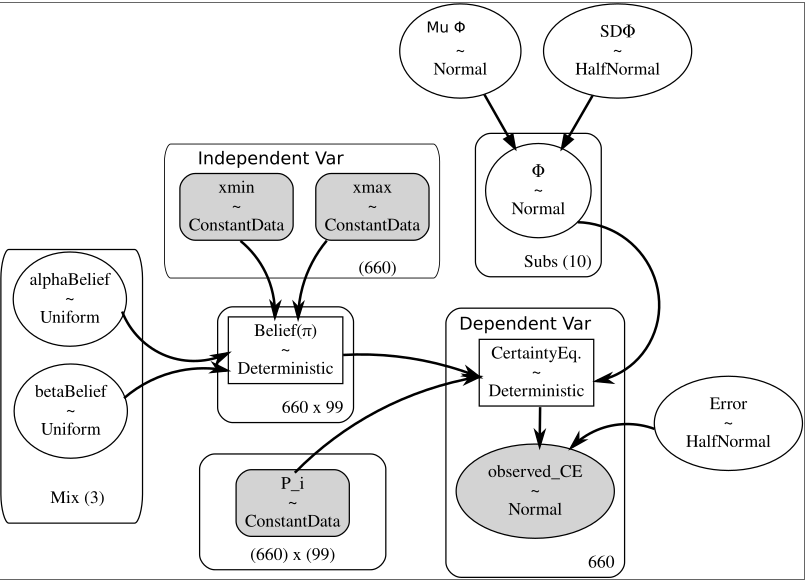
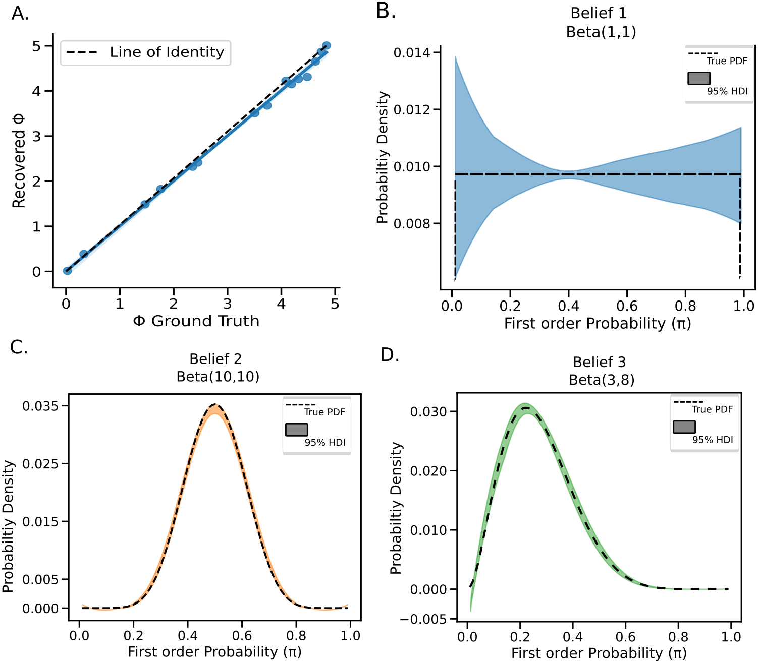
We run MCMC and see thatwe are able to recover both the phi parameters and the different beta distributions. Implemented with pymc
# ---------- Helper ----------
def beta_logp(values, alphas, betas):
    """Vectorized Beta logp with broadcasting"""
    dist = pm.Beta.dist(alpha=alphas, beta=betas)
    return pm.logp(dist, values)

# ---------- Model ----------
with pm.Model(coords=coords) as model:

    ##
    #-------------------------------------Input Data--------------------------------------------#
    ##
    sub_index   = pm.ConstantData("sub_index", sub_idx, dims="obs_id")
    tested_vals = pm.ConstantData("tested_vals", tested_vals_all, dims=("obs_id", "grid"))
    mix_index   = pm.ConstantData("mix_index", mix_idx, dims="obs_id")
    xmin   = pm.ConstantData("xmin", x_min, dims="obs_id")
    xmax   = pm.ConstantData("xmax", x_max, dims="obs_id")
    CE   = pm.ConstantData("ceobs", CEs, dims="obs_id")

    ##
    # ------------------- Belief Estimation with fences ---------------------------------------------#
    # Priors for the Belief
    alpha1 = pm.Uniform("alpha1", lower=0.5, upper=50, dims="Mix")
    beta1 = pm.Uniform("beta1", lower=0.5, upper=50, dims="Mix")
    # Shaping the parameters
    alpha1_obs = alpha1[mix_index][:, None]  # shape (n_obs,)
    beta1_obs  = beta1[mix_index][:, None]    # shape (n_obs,)

    #-------------------Calculate pi(p_)----------------------------------#
    pdf_vals = pm.math.exp(beta_logp(tested_vals, alpha1_obs, beta1_obs))

    pdf_vals = pm.math.where((tested_vals < xmin[:,None]) | (tested_vals > xmax[:,None]), 0, pdf_vals)

    norm_pdf = pm.Deterministic("normed_pdf", pdf_vals / pdf_vals.sum(axis=1, keepdims=True))

    #-------------------------------Utility Function and CE estimation----------------------------#

    #Priors for Utility
    #alpha_phi=pm.Uniform("alpha_phi",lower=0,upper=3)
    #beta_phi=pm.Uniform("beta_phi",lower=0,upper=3)
    #phi=pm.Weibull("phi",alpha=alpha_phi,beta=beta_phi,dims="Subs")
    mu_AA=pm.Normal("MUalpha",1,3)
    sd_AA=pm.HalfNormal("sd_AA",2)
    phi=pm.Normal("Φ", mu_AA,sd_AA,dims="Subs")

    #First round
    utility = pm.math.sum(
        ((10 * tested_vals)** phi[sub_index][:,None])*norm_pdf,
        axis=1)  # shape (n_obs,)
    #ce_e = pm.Deterministic("CE_exp", utility ** (1 / phi[sub_index]))
    ce_e = (utility ** (1 / phi[sub_index]))/10

    error = pm.HalfNormal("error", sigma=0.05)

    pm.Normal("observed_CE", mu=ce_e, sigma=error, observed=CE)

    # Sampling
    trace = pm.sample(draws=2000, tune=2000, chains=3, target_accept=0.95,nuts_sampler='nutpie')
| Parameter recovery | Model fit | Model convergence | |||
|---|---|---|---|---|---|
| Noise SD (σ) | R²($\hat{\phi}$, φ) | % Bias ($\hat{\phi}$ – φ)/φ | Posterior Predictive P-value | Mean $\hat{R}$ | Max $\hat{R}$ |
| 0.10 | 0.99 | 1.9% | 0.61 | 1.007 | 1.01 |